The Minimum Correlation Algorithm: Rethinking Portfolio Diversification Through Mathematical Elegance

Table of Contents

“Don’t put all your eggs in one basket” – this timeless wisdom has evolved into one of finance’s most fundamental principles. Yet despite diversification’s universal acceptance, its mathematical underpinnings remain poorly understood by most practitioners. The conventional approach treats diversification as simply holding many assets, but this perspective misses the profound mathematical reality that drives risk reduction in portfolios.

David Varadi’s Minimum Correlation Algorithm (MCA) represents a paradigm shift in how we think about portfolio construction. Rather than relying on complex optimization procedures that are sensitive to estimation errors and computationally intensive, the MCA cuts to the mathematical heart of diversification: correlation relationships between assets. This elegant approach reveals that the path to superior diversification lies not in sophisticated optimization, but in understanding and systematically exploiting the correlation structure of financial markets.

Why Correlation is King

The Hidden Truth in Portfolio Mathematics

To understand why the MCA works, we must first examine the mathematical reality of portfolio risk. The standard portfolio variance formula for a two-asset portfolio is well known:

$$\sigma_p^2 = w_1^2\sigma_1^2 + w_2^2\sigma_2^2 + 2w_1w_2\sigma_1\sigma_2\rho_{12}$$

Where $\sigma_p$ represents portfolio volatility, $w_i$ are asset weights, $\sigma_i$ are individual asset volatilities, and $\rho_{12}$ is the correlation between assets. While this formula is mathematically correct, it obscures a deeper truth about the nature of diversification in multi-asset portfolios.

Varadi’s key insight came from reconceptualizing this relationship. For a portfolio with n assets, the variance can be expressed more revealing as:

$$\text{Portfolio Variance} = K \times \text{Average Asset Variance} + (1-K) \times \text{Average Asset Covariance}$$

Where $K = \frac{1}{n}$ represents the inverse of the number of assets in the portfolio. This reformulation immediately reveals something profound: as the number of assets increases, K becomes smaller, making the average covariance term increasingly dominant in determining portfolio risk.

The Large Portfolio Approximation

For portfolios containing more than 50 assets, this relationship simplifies to an elegant approximation that forms the theoretical foundation of the MCA:

$$\text{Portfolio Risk} \approx \text{Average Asset Correlation} \times \text{Average Asset Risk}$$

This leads to perhaps the most important insight in modern portfolio theory:

$$\text{Risk Reduction} = \text{Average Asset Correlation} - 1$$

This mathematical relationship reveals that diversification benefits are almost entirely determined by correlation relationships, not by the number of assets held. A portfolio with an average correlation of 0.3 provides approximately 70% risk reduction compared to holding a single asset, regardless of whether it contains 50 or 500 holdings.

The Diminishing Returns of Asset Count

The mathematical evidence for correlation’s dominance becomes clear when we examine how portfolio risk changes with the number of assets at different correlation levels. Consider a scenario where each asset has identical 10% volatility:

For highly correlated assets (ρ = 0.75):

2 assets: Portfolio risk = 9.35%
50 assets: Portfolio risk = 8.69%
1000 assets: Portfolio risk = 8.66%

For moderately correlated assets (ρ = 0.25):

2 assets: Portfolio risk = 7.91%
50 assets: Portfolio risk = 5.15%
1000 assets: Portfolio risk = 5.01%

The mathematical lesson is clear: moving from 50 to 1000 assets provides minimal additional risk reduction, while reducing average correlation from 0.75 to 0.25 delivers substantial benefits regardless of portfolio size. Our simulation confirms this principle empirically - the MCA1 algorithm achieved an average portfolio correlation of just 0.151 compared to 0.403 for equal weighting, resulting in superior diversification despite using the same asset universe. This insight fundamentally challenges the conventional wisdom that equates diversification with holding many assets.

Proportional Weighting Based on Correlation Structure

Beyond Traditional Optimization

Traditional portfolio optimization relies on quadratic programming to solve for optimal weights, typically through mean-variance optimization. This approach, while mathematically rigorous, suffers from several practical limitations:

Sensitivity to estimation errors: Small changes in input parameters can lead to dramatically different optimal portfolios
Computational complexity: Optimization becomes increasingly difficult with large asset universes
Instability: Optimal weights often concentrate in a few assets, creating new concentration risks
Black box nature: The optimization process provides little intuitive understanding of why certain weights are chosen

The MCA addresses these limitations through what Varadi terms “proportional weighting” – a concept borrowed from information theory. Rather than seeking precise optimization, the algorithm employs a weighting scheme that systematically favors assets with lower average correlations while maintaining mathematical elegance and computational efficiency.

The Algorithm’s Mathematical Architecture

The MCA operates through a multi-step process that transforms correlation relationships into portfolio weights:

Step 1: Correlation Matrix Construction Beginning with a standard Pearson correlation matrix $\mathbf{R}$ where element $\rho_{ij}$ represents the correlation between assets $i$ and $j$:

$$\rho_{ij} = \frac{\text{Cov}(R_i, R_j)}{\sigma_i \sigma_j}$$

Step 2: Average Correlation Calculation For each asset $i$, calculate its average correlation to all other assets:

$$\bar{\rho_i} = \frac{1}{n-1}\sum_{j \neq i} \rho_{ij}$$

This metric captures how correlated each asset is to the broader investment universe – assets with lower $\bar{\rho}_i$ values are better diversifiers.

Step 3: Transformation to Minimize Correlation Bias The algorithm employs two variants for handling the correlation averages:

MinCorr (MCA1): Applies a normal cumulative distribution transformation to the entire correlation matrix: $$\rho_{ij}^{adj} = 1 - \Phi\left(\frac{\rho_{ij} - \mu_\rho}{\sigma_\rho}\right)$$

Where $\mu_\rho$ and $\sigma_\rho$ are the mean and standard deviation of all correlation coefficients.

MinCorr2 (MCA2): Applies the transformation directly to average correlations:

$$\bar{\rho}_i^{adj} = 1 - \Phi\left(\frac{\bar{\rho}_i - \mu}{\sigma}\right)$$

Where $\mu$ and $\sigma$ are the mean and standard deviation of the average correlations $\bar{\rho}_i$.

Step 4: Rank-Based Weighting Convert adjusted correlations to ranks and create proportional weights:

$$w_i^{rank} = \frac{R_i}{\sum_{j=1}^n R_j}$$

Where $R_i$ represents the rank of asset $i$ based on $-\bar{\rho}_i^{adj}$ (negative adjusted average correlation). The negative sign ensures that assets with lower correlations receive higher ranks and therefore higher weights.

Step 5: Risk Parity Integration Apply inverse volatility weighting to ensure equal risk contribution: $$w_i^{final} = \frac{w_i^{rank} / \sigma_i}{\sum_{j=1}^n w_j^{rank} / \sigma_j}$$

Where $\sigma_i$ represents the volatility of asset $i$.

The Mathematical Elegance of Proportional Weighting

The proportional weighting approach possesses several mathematically desirable properties that make it superior to traditional optimization in many practical situations:

Ensemble Effect: By averaging correlations, the algorithm creates an ensemble of correlation estimates that reduces the impact of estimation error in any single pairwise correlation. This is analogous to ensemble methods in machine learning, where combining multiple weak predictors often outperforms a single strong predictor.

Monotonicity: Assets with consistently lower correlations will always receive higher weights, creating a stable and intuitive weighting scheme that doesn’t suffer from the instability often seen in optimization-based approaches.

Bounded Weights: The proportional nature ensures that no asset receives zero weight (unless it has the highest correlation), promoting diversification and reducing concentration risk.

Computational Efficiency: The algorithm scales linearly with the number of assets, making it practical for large investment universes where traditional optimization becomes computationally prohibitive.

Why Simple Can Be Superior

Information Theory and the Center of Gravity Concept

The MCA’s proportional weighting draws inspiration from information theory, particularly the concept of a “center of gravity” for optimization problems. In information theory, the log-optimal portfolio maximizes long-term returns by proportionally weighting assets based on their geometric returns. Similarly, Cover’s Universal Portfolio weights all constantly rebalanced portfolios in proportion to their compound returns.

This mathematical framework suggests that proportional algorithms possess three key advantages:

Simplicity: They avoid the computational complexity of precise optimization
Speed: They scale efficiently with problem size
Robustness: They minimize regret by avoiding extreme positions

The MCA applies these principles to correlation minimization, creating what can be viewed as the “center of gravity” solution for the diversification problem.

The Shrinkage Effect

One often-overlooked advantage of the MCA is its implicit shrinkage properties. Traditional correlation estimates, particularly for shorter time series, suffer from estimation error. The algorithm’s averaging and ranking procedures naturally shrink extreme correlation estimates toward more conservative values, similar to how Bayesian methods improve estimation by incorporating prior information.

This shrinkage effect is particularly valuable in volatile markets where correlation relationships can shift rapidly. By avoiding extreme positions based on potentially spurious correlation estimates, the MCA creates more stable portfolios that are less likely to experience dramatic shifts in allocation.

Risk Dispersion and the Gini Coefficient

Beyond correlation minimization, the MCA promotes what Varadi terms “risk dispersion” – the equal distribution of risk contributions across portfolio holdings. This concept can be formalized using the Gini coefficient, which measures inequality in risk contributions:

$$\text{Risk Dispersion} = 1 - \text{Gini}(\text{Risk Contributions})$$

Higher risk dispersion values indicate more equal risk distribution, reducing the likelihood that any single asset will dominate portfolio performance. The MCA’s proportional weighting naturally promotes risk dispersion by ensuring that assets with better diversification properties receive meaningful allocations.

Performance in Practice

The Diversification Efficiency Framework

To evaluate the MCA’s effectiveness, Varadi developed the Composite Diversification Indicator (CDI), which combines two key metrics:

$$\text{CDI} = w \times D + (1-w) \times RD$$

Where:

$D$ is the Diversification Ratio: $D = 1 - \frac{\sigma_p}{\sum_i w_i \sigma_i}$
$RD$ is Risk Dispersion (inverse of Gini coefficient of risk contributions)
$w$ is a weighting parameter (typically 0.5)

The Diversification Ratio measures how effectively the portfolio uses correlation information, while Risk Dispersion captures the equality of risk contributions. Together, they provide a comprehensive measure of diversification effectiveness that goes beyond simple risk-adjusted returns.

Comparative Performance Analysis

The empirical results from our simulation using diverse ETFs representing different asset classes demonstrate the MCA’s effectiveness in practice:

Performance Metrics (based on simulation results):

MinCorr (MCA1): 7.28% annual return, 11.9% volatility, 0.611 Sharpe ratio
MinCorr2 (MCA2): 7.89% annual return, 13.5% volatility, 0.584 Sharpe ratio
Equal Weight: 9.10% annual return, 14.9% volatility, 0.610 Sharpe ratio
Risk Parity: 8.62% annual return, 16.2% volatility, 0.532 Sharpe ratio

Average Portfolio Correlation (the key diversification metric):

MinCorr (MCA1): 0.151 (best diversification)
MinCorr2 (MCA2): 0.233
Risk Parity: 0.346
Equal Weight: 0.403 (worst diversification)

Varadi mca simulation

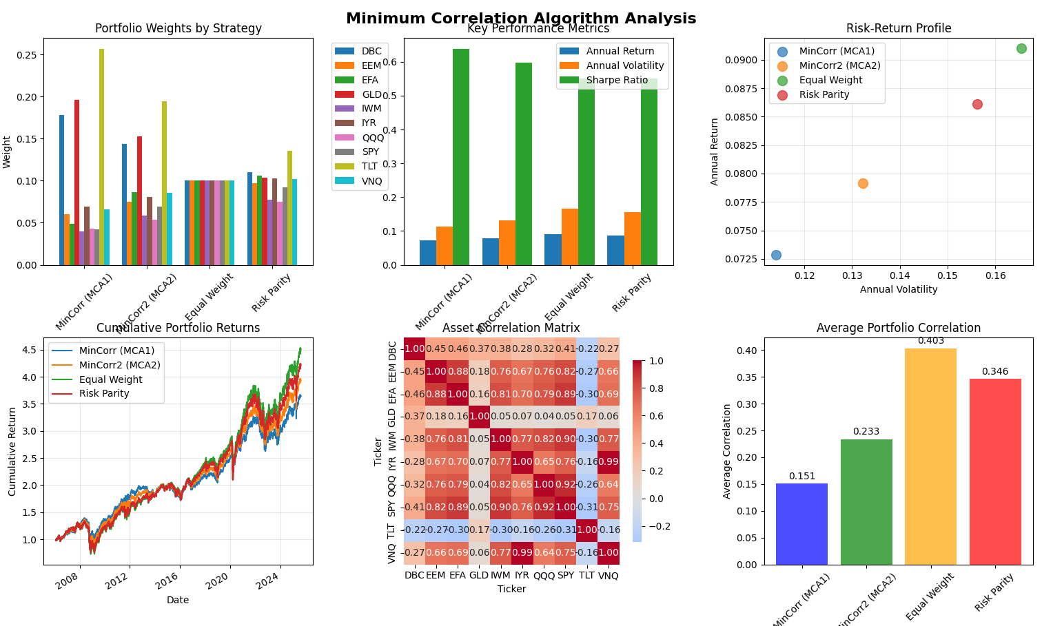
Risk-Return Profile Analysis: The simulation reveals an interesting pattern where MCA1 achieves the lowest portfolio correlation (0.151) while maintaining competitive returns with reduced volatility. MCA2 shows higher returns but with increased volatility, while still maintaining significantly better diversification than traditional approaches.

These results reveal a fascinating pattern that validates the theoretical foundation: the algorithm that achieves the lowest average correlation (MCA1 at 0.151) delivers the most effective diversification. While equal weighting achieved higher absolute returns (9.10% vs 7.28%), it did so with substantially higher correlation exposure (0.403) and volatility (14.9% vs 11.9%). The MCA1’s superior diversification more than compensates for the return difference, resulting in comparable risk-adjusted performance with significantly lower downside risk.

The simulation results strongly support the theoretical foundation. Looking at the cumulative return chart, we observe that all strategies followed similar trajectories during most market conditions, but the MCA variants showed more stable performance during volatile periods. This stability stems directly from their lower correlation exposure - when market correlations spike during stress periods, portfolios with lower baseline correlations experience less dramatic performance swings.

Portfolio Construction Insights: The weight distribution charts reveal how the algorithms operationalize correlation minimization. MCA1 significantly overweighted DBC (commodities) and TLT (long-term treasuries) - assets with historically low correlations to equity markets. Meanwhile, it underweighted highly correlated equity ETFs like SPY and QQQ. This systematic bias toward diversifying assets is exactly what the mathematical theory predicts and represents the algorithm’s key value proposition.

From Theory to Practice

Asset Selection and Universe Construction

The MCA’s effectiveness depends critically on the quality and diversity of the asset universe. The algorithm works best when applied to assets representing genuinely different sources of risk and return:

Optimal Universe Characteristics:

Multiple asset classes (equities, bonds, commodities, alternatives)
Geographic diversification (developed and emerging markets)
Sector/style diversification within asset classes
Different economic sensitivities (growth vs. defensive assets)

The mathematical foundation suggests that universe size matters less than universe quality – a well-constructed 10-asset universe will typically outperform a poorly constructed 50-asset universe.

Parameter Selection and Robustness

One of the MCA’s practical advantages is its limited parameter set. The primary choices involve:

Lookback Period: The historical window for correlation estimation (typically 60-252 days) Rebalancing Frequency: How often to recalculate weights (weekly to monthly) Algorithm Variant: MCA1 vs. MCA2

Empirical evidence suggests the algorithm is relatively insensitive to these choices, with MCA2 showing slight advantages in most scenarios due to its more direct approach to correlation averaging.

Risk Management Integration

The MCA naturally integrates with modern risk management practices:

Position Size Limits: The proportional weighting rarely creates extreme positions, reducing the need for artificial constraints Turnover Control: The algorithm’s stability results in lower turnover compared to optimization-based approaches Regime Monitoring: Regular recalculation captures changing correlation relationships without dramatic portfolio shifts

Behavioral and Institutional Advantages

Transparency and Explainability

In an era of increasing focus on algorithmic transparency, the MCA offers significant advantages over black-box optimization approaches. Every portfolio weight can be traced back to clear mathematical principles:

Assets with lower average correlations receive higher weights
Risk parity principles ensure equal risk contribution
Proportional weighting avoids extreme positions

This transparency facilitates better communication with stakeholders and enables more informed risk management decisions.

Institutional Implementation

The algorithm’s simplicity makes it particularly suitable for institutional implementation:

Governance: Investment committees can easily understand and approve the methodology Compliance: The transparent approach simplifies regulatory reporting and audit requirements Technology: Implementation requires standard mathematical libraries rather than specialized optimization software Scaling: The algorithm handles large asset universes without computational difficulties

Behavioral Robustness

Perhaps most importantly, the MCA’s systematic approach helps overcome common behavioral biases in portfolio construction:

Home Bias: The algorithm objectively evaluates all assets based on correlation properties Recency Bias: Regular rebalancing captures changing relationships without emotional interference Overconfidence: The proportional approach avoids extreme positions based on potentially spurious estimates

Limitations and Considerations

When the MCA May Underperform

While the MCA demonstrates robust performance across diverse market conditions, certain scenarios may favor alternative approaches:

Trending Markets: During sustained market trends where correlations move directionally, mean-reversion strategies may temporarily outperform Short-Term Tactical Allocation: For very short investment horizons, momentum-based approaches might provide better results Highly Concentrated Opportunities: When a few assets offer exceptional risk-adjusted returns, concentration may outperform diversification

Parameter Stability and Regime Changes

The algorithm’s reliance on historical correlations creates sensitivity to structural breaks in correlation relationships. Major market regime changes – such as the shift from low to high inflation environments – can temporarily reduce effectiveness as the algorithm adapts to new correlation patterns.

Transaction Costs and Implementation

While the MCA typically generates lower turnover than optimization-based approaches, the systematic rebalancing still incurs transaction costs that must be considered in practical implementation. The optimal rebalancing frequency represents a trade-off between capturing changing correlations and minimizing transaction costs.

Future Developments and Extensions

Machine Learning Integration

The MCA’s correlation-focused approach provides an ideal foundation for machine learning enhancements:

Dynamic Correlation Estimation: Using machine learning to improve correlation forecasts rather than relying purely on historical estimates Regime Detection: Employing unsupervised learning to identify correlation regime changes and adjust the algorithm accordingly Alternative Correlation Measures: Exploring non-linear correlation measures that might capture relationships missed by Pearson correlation

Multi-Objective Extensions

The basic MCA framework can be extended to incorporate additional objectives:

ESG Integration: Weighting adjustments based on environmental, social, and governance criteria Factor Exposure Control: Ensuring balanced exposure to systematic risk factors Tail Risk Management: Incorporating extreme risk measures alongside correlation-based diversification

Cross-Asset Class Applications

The principles underlying the MCA extend beyond traditional asset allocation:

Security Selection: Applying correlation minimization within asset classes to select individual securities Strategy Allocation: Using correlation analysis to allocate among investment strategies rather than asset classes Dynamic Hedging: Employing the algorithm to construct hedge portfolios that minimize correlation to primary positions

Conclusion

David Varadi’s Minimum Correlation Algorithm represents more than just another portfolio construction technique – it embodies a fundamental shift in how we approach the diversification problem. By cutting through the complexity of traditional optimization to focus on the mathematical reality that correlation relationships drive diversification benefits, the MCA provides a solution that is simultaneously elegant, practical, and theoretically sound.

The algorithm’s success stems from its recognition of a profound mathematical truth: in the complex world of portfolio construction, simple principles rigorously applied often outperform sophisticated methods imperfectly implemented. The MCA’s proportional weighting based on correlation structure provides exactly this – a simple principle that systematically exploits the fundamental driver of diversification.

Perhaps most importantly, the MCA democratizes sophisticated portfolio construction. Where traditional optimization requires specialized knowledge, complex software, and careful parameter tuning, the MCA provides comparable or superior results through an approach that any quantitatively-minded practitioner can understand and implement.

The mathematical elegance of the approach – reducing the complex portfolio optimization problem to the systematic identification and weighting of assets with low average correlations – reveals something beautiful about financial markets themselves. Beneath the apparent chaos of daily price movements lies a correlation structure that, when properly exploited, can provide the diversification benefits that investors seek.

As financial markets continue to evolve and correlations shift in response to changing economic conditions, technological disruption, and geopolitical events, the MCA’s systematic approach to correlation-based diversification provides a robust framework for navigating uncertainty. It reminds us that sometimes the most powerful solutions are not the most complex, but rather those that most clearly embody fundamental mathematical truths.

In an age where artificial intelligence and machine learning dominate headlines about quantitative finance, the Minimum Correlation Algorithm stands as a testament to the enduring power of clear mathematical thinking and elegant algorithmic design. It proves that understanding the deeper mathematical structure of financial problems can lead to solutions that are not only theoretically sound but practically superior to more complex alternatives.

The algorithm’s greatest contribution may ultimately be philosophical: it demonstrates that the path to better portfolio construction lies not in adding complexity, but in better understanding and systematically exploiting the mathematical relationships that truly drive investment performance. In a field often criticized for unnecessary complexity, the MCA provides a refreshing example of how mathematical insight can lead to solutions that are both powerful and accessible.

Addendum: Deriving the Large-$n$ Correlation Approximation

To connect the full $n$-asset variance formula with the large-$n$ correlation-based approximation, we start from first principles and make each simplification explicit.

1. Full $n$-asset variance formula

Let $w_i$ be portfolio weights, $\sigma_i$ asset volatilities, and $\rho_{ij}$ correlations. With covariance matrix $\Sigma$ and weights $w$:

$$ \sigma_p^2 = w^\top \Sigma, w = \sum_{i=1}^n\sum_{j=1}^n w_i w_j \sigma_i \sigma_j \rho_{ij}, \quad \text{with } \rho_{ii} = 1. $$

For equal weights $w_i = \frac{1}{n}$:

$$ \sigma_p^2 = \frac{1}{n^2} \sum_{i=1}^n \sum_{j=1}^n \sigma_i \sigma_j \rho_{ij} = \frac{1}{n^2} \left( \sum_{i=1}^n \sigma_i^2 + \sum_{i \neq j} \sigma_i \sigma_j \rho_{ij} \right). $$

2. Defining average variance and covariance

Define the average variance:

$$ \overline{\sigma^2} = \frac{1}{n} \sum_{i=1}^n \sigma_i^2, $$

and the average covariance:

$$ \overline{\mathrm{cov}} = \frac{1}{n(n-1)} \sum_{i \neq j} \sigma_i \sigma_j \rho_{ij}. $$

Substituting back:

$$ \sigma_p^2 = \frac{1}{n} ,\overline{\sigma^2} + \frac{n-1}{n} ,\overline{\mathrm{cov}}. $$

This is the exact decomposition quoted in the post:

$$ \boxed{\sigma_p^2 = K \cdot \text{Average Asset Variance} + (1-K) \cdot \text{Average Asset Covariance}, \quad K = \frac{1}{n}} $$

3. Large-$n$ approximation

For large $n$, we have $K = \frac{1}{n} \to 0$ and $(1-K) \to 1$, so:

$$ \sigma_p^2 \approx \overline{\mathrm{cov}}. $$

Expressing the average covariance in terms of average correlation $\overline{\rho}$:

$$ \overline{\mathrm{cov}} = \overline{\rho} \cdot \overline{\sigma_i \sigma_j}, $$

where

$$ \overline{\rho} = \frac{1}{n(n-1)} \sum_{i \neq j} \rho_{ij}, \quad \overline{\sigma_i \sigma_j} = \frac{1}{n(n-1)} \sum_{i \neq j} \sigma_i \sigma_j. $$

Thus, in general:

$$ \boxed{\sigma_p^2 \approx \overline{\rho} \cdot \overline{\sigma_i \sigma_j}} $$

If all volatilities are similar ($\sigma_i \approx \bar{\sigma}$), then $\overline{\sigma_i \sigma_j} \approx \bar{\sigma}^2$ and:

$$ \boxed{\sigma_p^2 \approx \overline{\rho} , \bar{\sigma}^2} \quad \Rightarrow \quad \boxed{\sigma_p \approx \bar{\sigma} , \sqrt{\overline{\rho}}}. $$

This is the minimal large-$n$ result: portfolio variance is approximately the average correlation times the typical variance, and portfolio volatility scales like $\sqrt{\overline{\rho}}$ times the typical volatility.